An annotated guide to the Kolmogorov-Arnold Network
if the LaTeX is not loading, refresh the page.
This post is analogous to and heavily inspired by the Annotated Transformer but for KANs. It is fully functional as a standalone notebook, and provides intuition along with the code. Most of the code was written to be easy to follow and to mimic the structure of a standard deep learning model in PyTorch, but some parts like training loops and visualization code were adapted from the original codebase. We decided to remove some sections from the original paper that were deemed unimportant, and also includes some extra works to motivate future research on these models.
The original paper is titled “KAN: Kolmogorov-Arnold Networks”, and the authors on this paper are: Ziming Liu, Yixuan Wang, Sachin Vaidya, Fabian Ruehle, James Halverson, Marin Soljačić, Thomas Y. Hou, and Max Tegmark.
Introduction
Deep neural networks have been the driving force of developments in AI in the last decade. However, they currently suffer from several known issues such as a lack of interpretability, scaling issues, and data inefficiency – in other words, while they are powerful, they are not a perfect solution.
Kolmogorov-Arnold Networks (KANs) are an alternative representation to standard multi-layer perceptrons (MLPs). In short, they parameterize activation functions by re-wiring the “multiplication” in an MLP’s weight matrix-vector multiplication into function application. While KANs are not nearly as provably accomplished as MLPs, they are an exciting prospect for the field of AI and deserve some time for exploration.
I have separated this article into two sections. Parts I & II describe a minimal KAN architecture and training loop without an emphasis on B-spline optimizations. You can use the minimal KAN notebook if you’re interested in KANs at a high-level. Parts III & IV describe B-spline specific optimizations and an application of KANs, which includes a bit of extra machinery in the KAN code. You can use the full KAN notebook if you want to follow along there.
Background and Motivation
Before jumping into the implementation details, it is important to take a step back and understand why one should even care about these models. It is quite well known that Multi-layer Perceptrons (MLPs) have the “Universal Approximation Theorem”, which provides a theoretical guarantee for the existence of an MLP that can approximate any functionThis is a very strong guarantee that usually isn't actually true. Generally, we have some provable guarantee for a class of functions that we actually care about approximating, like say the set of functions in L1 or the set of smooth, continuous functions. up to some error \(\epsilon\). While this guarantee is important, in practice, it says nothing about how difficult it is to find such an MLP through, say, optimization with stochastic gradient descent.
KANs admit a similar guarantee through the Kolmogorov-Arnold representation theorem, though with a caveatSee section [Are Stacked KAN Layers a Universal Approximator?]. Formally, the theorem states that for a set of covariates \((x_1,x_2,...,x_n)\), we can write any continuous, smoothSmooth in this context means in $C^{\infty}$, or infinitely differentiable. function \(f(x_1,...,x_n) : \mathcal{D} \rightarrow \mathbb{R}\) over a bounded domain \(\mathcal{D}\)Because it is bounded, the authors argue that we can normalize the input to the space $[0,1]^{n}$, which is what is assumed in the original paper. in the form
where \(\Phi_{q,p}, \Phi_{q}\) are univariate functions from \(\mathbb{R}\) to \(\mathbb{R}\). In theory, we can parameterize and learn these (potentially non-smooth and highly irregular) univariate functions \(\Phi_{q,p}, \Phi_{q}\) by optimizing a loss function similar to any other deep learning model. But it’s not that obvious how one would “parameterize” a function the same way you would parameterize a weight matrix. For now, just assume that it is possible to parameterize these functions – the original authors choose to use a B-spline, but there is little reason to be stuck on this choice.
What is a KAN?
The expression from the theorem above does not describe a KAN with $L$ layers. This was an initial point of confusion for me. The universal approximation guarantee is only for models specifically in the form of the Kolmogorov-Arnold representation, but currently we have no notion of a “layer” or anything scalable. In fact, the number of parameters in the above theorem is a function of the number of covariates and not the choice of the engineer! Instead, the authors define a KAN layer \(\mathcal{K}_{m,n}\) with input dimension \(n\) and output dimension \(m\) as a parameterized matrix of univariate functions, \(\Phi = \{\Phi_{i,j}\}_{i \in [m], j \in [n]}\).
It may seem like the authors pulled this expression out of nowhere, but it is easy to see that the KAN representation theorem can be re-written as follows. For a set of covariates \(\boldsymbol{x} = (x_1,x_2,...,x_n)\), we can write any continuous, smooth function \(f(x_1,...,x_n) : \mathcal{D} \rightarrow \mathbb{R}\) over a bounded domain \(\mathcal{D}\) in the form
The KAN architecture, is therefore written as a composition of stacking these KAN layers, similar to how you would compose an MLP. I want to emphasize that unless the KAN is written in the form above, there is currently no provenI suspect that there are some provable guarantees that can be made for deep KANs. The original universal approximation theorem for MLPs refers to models with a single hidden dimension, but later works have also derived guarantees for deep MLPs. We also technically don't have very strong provable guarantees for mechanisms like self-attention (not to my knowledge at least), so I don't think it's that important in predicting the usefulness of KANs. theoretical guarantee that there exists a KAN represents that approximates the desired function.
Are Stacked KAN Layers a Universal Approximator?
When first hearing about KANs, I was under the impression that the Kolmogorov-Arnold Representation Theorem was an analogous guarantee for KANs, but this is seemingly not true. Recall from the Kolmogorov-Arnold representation theorem that our guarantee is only for specific 2-layer KAN models. Instead, the authors prove that there exists a KAN using B-splines as the univariate functions \(\{\Phi_{i,j}\}_{i \in [m], j \in [n]}\) that can approximate a composition of continuously-differentiable functions within some nice error marginThis article serves mainly as a concept to code guide, so I didn't want to dive too much into theory. The error bound that the authors prove is quite strange, as the constant $C$ is not *really* a constant in the traditional sense (it depends on the function you are approximating). Also, the function family they choose to approximate seems pretty general, but I'm actually not that sure what types of functions it cannot represent well. I'd recommend reading Theorem 2.1 on your own, but it mainly serves as justification for the paper's use of B-splines rather than a universal approximation theorem for generic KAN networks. . Their primary guarantees are proven to justify the use of B-splines as their learnable activations, but other works have recently sprung up that propose different learnable activations like Chebyshev polynomials, RBFs , and wavelet functions .
tldr; no, we have not shown that a generic KAN model serves as the same type of universal approximator as an MLP (yet).
Polynomials, Splines, and B-Splines
We talked quite extensively about “learnable activation functions”, but this notion might be unclear to some readers. In order to parameterize a function, we have to define some kind of “base” function that uses coefficients. When learning the function, we are actually learning the coefficients. The original Kolmogorov-Arnold representation theorem places no conditions on the family of learnable univariate activation functions. Ideally, we would want some kind of parameterized family of functions that can approximate any function, whether it be non-smooth, fractal, or some other kind of nasty property on a bounded domainNot only is the original KAN representation theorem over a bounded domain, but generally in most practical applications we are not dealing with data over an unbounded domain..
Enter the B-spline. B-splines are a generalization of spline functions, which themselves are piecewise polynomials. Polynomials of degree/order \(k\) are written as \(p(x) = a_0 + a_1x + a_2x^2 + ... + a_kx^k\) and can be parameterized according to their coefficients \(a_0,a_1,...,a_k\). From the Stone-Weierstrass theorem , we can guarantee that every continuous function over a bounded domain can be approximated by a polynomial. Splines, and by extension B-splines, extend this guarantee to more complicated functions over a bounded domain. I don’t want to take away from the focus on KANs, so for more background I’d recommend reading this resource.
Rather than be chunked explicitly like a spline, B-spline functions are written as a sum of basis functions of the form
where \(G\) denotes the number of grid points and therefore basis functions (which we have not defined yet), $k$ is the order of the B-spline, and \(c_i\) are learnable parameters. Like a spline, a B-spline has a set of $G$ grid pointsThese are also called knots. B-splines are determined by control points, which are the data points we're trying to fit. Sometimes knots and control points can be the same, but generally knots are fixed beforehand and can be adjusted. \((t_1,t_2,...,t_G)\). In the KAN paper, they augment these points to \((t_{-k}, t_{-k+1},...,t_{G+k-1},t_{G+k})\) to account for the order of the B-spline Read https://web.mit.edu/hyperbook/Patrikalakis-Maekawa-Cho/node17.html for a better explanation for why you need to do this. It is mainly so the basis functions are well defined. to give us an augmented grid size of \(G+2k\). The simplest definition for the grid points is to uniformly divide the bounded domain into $G$ equally spaced points – from our definition of the basis functions, you will see that the augmented points just need to be at the ends. The Cox-de Boor formula characterizes these basis functions recursively as follows:
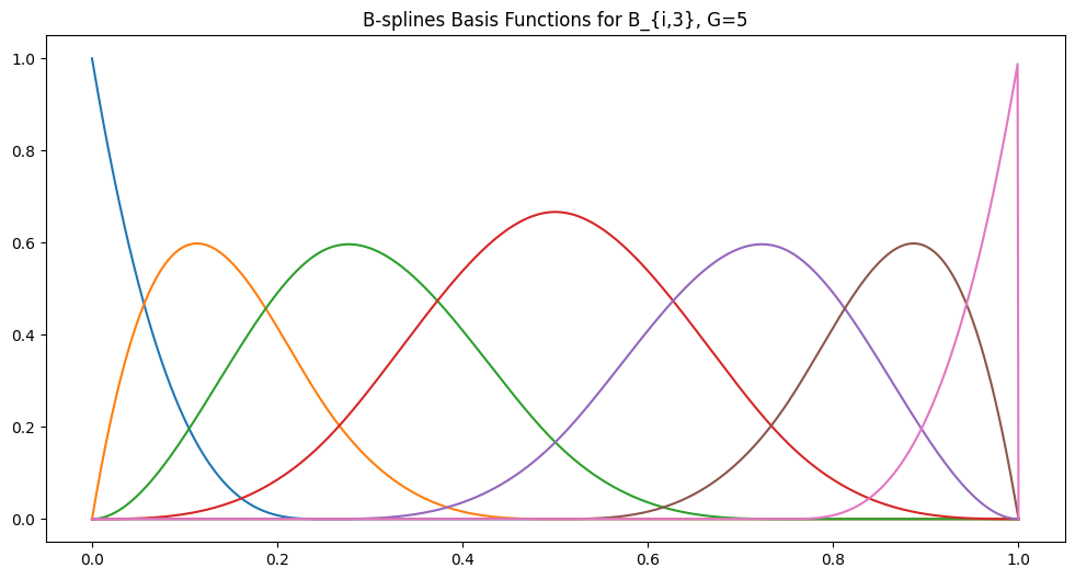
We can plot an example for the basis functions of a B-spline with $G=5$ grid points of order $k=3$. In other words, the augmented grid size is $G+2k=11$:
Matplotlib plot of B-spline basis functions. Notably, the basis functions, like spline polynomials, are $0$ on most of the domain. But they overlap, unlike for splines. I generated this graph by adapting code from https://github.com/johntfoster/bspline/.
When implementing B-splines for our KAN, we are not interested in the function \(f(\cdot)\) itself, rather we care about efficiently computing the function evaluated at a point \(f(x)\). We will later see a nice iterative bottom-up dynamic programming formulation of the Cox-de Boor recursion.
Part I: The Minimal KAN Model Architecture
In this section, we describe a barebones, minimal KAN model. The goal is to show that the architecture is structured quite similarly to deep learning code that the reader has most likely seen in the past. To summarize the components, we modularize our code into (1) a high-level KAN module, (2) the KAN layer, (3) the parameter initialization scheme, and (4) the plotting function for interpreting the model activations.
Preliminaries
If you’re using Colab, you can run the following as if they were code blocks. This implementation is also quite GPU-unfriendly, so a CPU will suffice.
# Code was written in Python 3.11.9, but most usable versions of Python and torch suffice.
!pip install torch==2.3.1
!pip install numpy==1.26.4
!pip install matplotlib==3.9.0
!pip install tqdm==4.66.4
!pip install torchvision==0.18.1
In an attempt to make this code barebones, I’ve tried to use as little dependencies as possible. I’ve also included type annotations for the code.
# Python libraries
import os
from typing import List, Dict, Optional, Self
import random
import warnings
# Installed libraries
import torch
import torch.nn as nn
import torch.nn.functional as F
from torchvision import datasets, transforms
import numpy as np
import matplotlib.pyplot as plt
from tqdm import tqdm
The following config file holds some preset hyperparameters described in the paper. Most of these can be changed and may not even apply to a more generic KAN architecture.
class KANConfig:
"""
Configuration struct to define a standard KAN.
"""
residual_std = 0.1
grid_size = 5
spline_order = 3
grid_range = [-1.0, 1.0]
device = torch.device("cuda" if torch.cuda.is_available() else "cpu")
The KAN Architecture Skeleton
If you understand how MLPs work, then the following architecture should look familiar. As always, given some set of input features \((x_1,...,x_n)\) and a desired output \((y_1,...,y_m)\), we can think of our KAN as a function \(f : \mathbb{R}^{n} \rightarrow \mathbb{R}^{m}\) parameterized by weights \(\theta\). Like any other deep learning model, we can decompose KANs in a layer-wise fashion and offload the computational details to the layer class. We will fully describe our model in terms of a list of integers layer_widths, where the first number denotes the input dimension \(n\), and the last number denotes the output dimension \(m\).
class KAN(nn.Module):
"""
Standard architecture for Kolmogorov-Arnold Networks described in the original paper.
Layers are defined via a list of layer widths.
This minimal implementation doesn't include optimizations used specifically
for B-splines.
"""
def __init__(
self,
layer_widths: List[int],
config: KANConfig,
):
super(KAN, self).__init__()
self.layers = torch.nn.ModuleList()
self.layer_widths = layer_widths
# If layer_widths is [2,4,5,1], the layer
# inputs are [2,4,5] and the outputs are [4,5,1]
in_widths = layer_widths[:-1]
out_widths = layer_widths[1:]
for in_dim, out_dim in zip(in_widths, out_widths):
self.layers.append(
KANLayer(
in_dim=in_dim,
out_dim=out_dim,
grid_size=config.grid_size,
spline_order=config.spline_order,
device=config.device,
residual_std=config.residual_std,
grid_range=config.grid_range,
)
)
def forward(self, x: torch.Tensor):
"""
Standard forward pass sequentially across each layer.
"""
for layer in self.layers:
x = layer(x)
return x
The KAN Representation Layer
The representation used at each layer is quite intuitive. For an input \(x \in \mathbb{R}^{n}\), we can directly compare a standard MLP layer with output dimension \(m\) to an equivalent KAN layer:
$$
\begin{aligned}
h_{MLP} = \sigma (W \boldsymbol{x} + b) \quad \quad &\text{ where } \quad \quad \forall i \in [m], (W\boldsymbol{x})_{i} = \sum_{k=1}^n W_{i,k} x_k
\\
h_{KAN} = \Phi \boldsymbol{x} + b \quad \quad &\text{ where } \quad \quad \forall i \in [m], (\Phi \boldsymbol{x})_{i} = \sum_{k=1}^n \Phi_{i,k} (x_k)
\end{aligned}
$$
In other words, both layers can be written in terms of a generalized matrix-vector operation, where for an MLP it is scalar multiplication, while for a KAN it is some learnable non-linear function \(\Phi_{i,k}\). Interestingly, both layers look extremely similar! Remark. As a GPU enthusiast, I should mention that while these two expressions look quite similar, this minor difference can have a huge impact on efficiency. Having the same instruction (e.g. multiplication) applied to every operation fits well within the warp abstraction used in writing CUDA kernels, while having a different function application per operation has many issues like control divergence that significantly slow down performance.
Let’s think through how we would perform this computation. For our analysis, we will ignore the batch dimension, as generally this is an easy extension. Suppose we have a KAN layer \(\mathcal{K}_{m,n}\) with input dimension\(n\) and output dimension \(m\). As we discussed earlier, for input \((x_1,x_2,...,x_n)\),
The observant reader may notice that this looks exactly like the $Wx$ matrix used in an MLP. In other words, we have to compute and materializeFor convenience sake, we will materialize the matrix of values below all at once. I suspect that, similar to matrix multiplication, there may be a way to avoid materializing the full matrix all at once, but this requires a clever choice of the family of functions for $\Phi$. each term in the matrix below, then sum along the rows.
$$
\text{The terms we need to compute are }
\begin{bmatrix}
\Phi_{1,1}(x_1), \Phi_{1,2}(x_2), ..., \Phi_{1,n}(x_n) \\
\Phi_{2,1}(x_1), \Phi_{2,2}(x_2), ...,\Phi_{2,n}(x_n) \\
\vdots \\
\Phi_{m,1}(x_1), \Phi_{m,2}(x_2), ..., \Phi_{m,n}(x_n) \\
\end{bmatrix}
$$
To finish off the abstract KAN layer (remember, we haven’t defined what the learnable activation function is), the authors define each learnable activation function $\Phi_{i,j}(\cdot)$ as a function of a learnable activation function $s_{i,j}(\cdot)$ to add residual connections in the network:
We can modularize the operation above into a “weighted residual layer” that acts over a matrix of \((\text{out_dim}, \text{in_dim})\) values. This layer is parameterized by each \(w^{(b)}_{i,j}\) and \(w^{(s)}_{i,j}\), so we can store \(\boldsymbol{w}^{(b)}\) and \(\boldsymbol{w}^{(s)}\) as parameterized weight matrices. The paper also specifies the initialization scheme of \(w^{(b)}_{i,j} \sim \mathcal{N}(0, 0.1)\) and \(w^{(s)}_{i,j} = 1\).For all the code comments below, I notate `bsz` as the batch size. Generally, this is just an extra dimension that can be ignored during the analysis.
class WeightedResidualLayer(nn.Module):
"""
Defines the activation function used in the paper,
phi(x) = w_b SiLU(x) + w_s B_spline(x)
as a layer.
"""
def __init__(
self,
in_dim: int,
out_dim: int,
residual_std: float = 0.1,
):
super(WeightedResidualLayer, self).__init__()
self.univariate_weight = torch.nn.Parameter(
torch.Tensor(out_dim, in_dim)
) # w_s in paper
# Residual activation functions
self.residual_fn = F.silu
self.residual_weight = torch.nn.Parameter(
torch.Tensor(out_dim, in_dim)
) # w_b in paper
self._initialization(residual_std)
def _initialization(self, residual_std):
"""
Initialize each parameter according to the original paper.
"""
nn.init.normal_(self.residual_weight, mean=0.0, std=residual_std)
nn.init.ones_(self.univariate_weight)
def forward(self, x: torch.Tensor, post_acts: torch.Tensor):
"""
Given the input to a KAN layer and the activation (e.g. spline(x)),
compute a weighted residual.
x has shape (bsz, in_dim) and act has shape (bsz, out_dim, in_dim)
"""
# Broadcast the input along out_dim of post_acts
res = self.residual_weight * self.residual_fn(x[:, None, :])
act = self.univariate_weight * post_acts
return res + act
With these operations laid out in math, we have enough information to write a basic KAN layer by abstracting away the choice of learnable activation \(s_{i,j}(\cdot)\). Note that in the code below, the variables spline_order, grid_size, and grid_range are specific to B-splines as the activation, and are only passed through the constructor. You can ignore them for now. In summary, we will first compute the matrix
following by the weighted residual across each entry, then we will finally sum along the rows to get our layer output. We also define a cache() function to store the input vector \(\boldsymbol{x}\) and the \(\Phi \boldsymbol{x}\) matrix to compute regularization terms defined later.
class KANLayer(nn.Module):
"Defines a KAN layer from in_dim variables to out_dim variables."
def __init__(
self,
in_dim: int,
out_dim: int,
grid_size: int, # B-spline parameter
spline_order: int, # B-spline parameter
device: torch.device,
residual_std: float = 0.1,
grid_range: List[float] = [-1, 1], # B-spline parameter
):
super(KANLayer, self).__init__()
self.in_dim = in_dim
self.out_dim = out_dim
self.grid_size = grid_size
self.spline_order = spline_order
self.device = device
# Define univariate function (splines in original KAN)
self.activation_fn = KANActivation(
in_dim,
out_dim,
spline_order,
grid_size,
device,
grid_range,
)
# Define the residual connection layer used to compute \phi
self.residual_layer = WeightedResidualLayer(in_dim, out_dim, residual_std)
# Cache for regularization
self.inp = torch.empty(0)
self.activations = torch.empty(0)
def cache(self, inp: torch.Tensor, acts: torch.Tensor):
self.inp = inp
self.activations = acts
def forward(self, x: torch.Tensor):
"""
Forward pass of KAN. x is expected to be of shape (bsz, in_dim) where in_dim
is the number of input scalars and the output is of shape (bsz, out_dim).
"""
# Compute each s_{i,j}, shape: [bsz x out_dim x in_dim]
spline = self.activation_fn(x)
# Form the batch of matrices phi(x) of shape [bsz x out_dim x in_dim]
phi = self.residual_layer(x, spline)
# Cache activations for regularization during training.
self.cache(x, phi)
# Really inefficient matmul
out = torch.sum(phi, dim=-1)
return out
KAN Learnable Activations: B-Splines
Recall from the section on B-splines that each activation $s_{i,j}(\cdot)$ is a sum of productsWe can equivalently think of this as a dot product between two vectors $\langle c_{i,j}, B_{i,j} (x_j) \rangle$. of $G + k$ learnable coefficients and basis functions \(\sum_{h=1}^{G} c^{h}_{i,j}, B^h_{i,j} (x_j)\) where $G$ is the grid size. The recursive definition of the B-spline basis functions requires us to define the grid points $(t_1,t_2,…,t_G)$, as well as the augmented grid points \((t_{-k},t_{-k+1},...,t_{-1},t_{G+1},....,t_{G+k})\)In the original paper, you may have noticed a G + k - 1 term. I don't define $t_0$ here, and opt to not include it for indexing sake, but you can basically just shift everything by $1$ to achieve the same effect.. For now, we will define them to be the endpoints of $G+1$ equally-sized intervals on the bounded interval [low_bound, up_bound]I mentioned this earlier, but you may notice that the augmented grid points go out of the bounded domain. This is just for convenience, but as long as they are at the bounds or outside them in the right direction, it doesn't matter what they are. You can also just set them to be the boundary points. but you can also choose / learn the grid point positions. Finally, we note that we need to use the grid points in the calculation of each activation $s_{i,j}(x)$, so we broadcast into a 3D tensor.
def generate_control_points(
low_bound: float,
up_bound: float,
in_dim: int,
out_dim: int,
spline_order: int,
grid_size: int,
device: torch.device,
):
"""
Generate a vector of {grid_size} equally spaced points in the interval
[low_bound, up_bound] and broadcast (out_dim, in_dim) copies.
To account for B-splines of order k, using the same spacing, generate an additional
k points on each side of the interval. See 2.4 in original paper for details.
"""
# vector of size [grid_size + 2 * spline_order + 1]
spacing = (up_bound - low_bound) / grid_size
grid = torch.arange(-spline_order, grid_size + spline_order + 1, device=device)
grid = grid * spacing + low_bound
# [out_dim, in_dim, G + 2k + 1]
grid = grid[None, None, ...].expand(out_dim, in_dim, -1).contiguous()
return grid
Again recall the Cox-de Boor recurrence from before.
As a general rule of thumb we would like to avoid writing recurrent functions in the forward pass of a model. A common trick is to turn our recurrence into a dynamic-programming solution, which we make clear by writing in array notation:
The tricky part is writing this in tensor notationI'd recommend drawing this out yourself. It's quite hard to explain without visualizations, but quite simple to reason about. . We take advantage of broadcasting rules in PyTorch/Numpy to make copies of tensors when needed. Recall that to materialize our activation matrix \(\{s_{i,j}(x_j)\}_{i \in [m], j \in [n]}\) we need to compute the bases for each activation, i.e. \(\{B^{(i,j)}_{h,k} (x_j)\}_{h \in [G+k], i \in [m], j \in [n]}\).
The following explanation is a bit verbose, so bear with me. Our grid initialization function above generates a rank-3 tensor of shape (out_dim, in_dim, G+2k+1) while the input $x$ is a rank-2 tensor of shape (batch_size, in_dim). We first notice that our grid applies to every input in the batch, so we broadcast it to a rank-4 tensor of shape (batch_size, out_dim, in_dim, G+2k+1). For the input $x$, we similarly need a copy for every output dimension and every basis function to evaluate over, giving us the same shape through broadcasting. We can align the in_dim axis of both the grid and the input because $j$ aligns in $s_{i,j}(x_j)$. The $i$ indexes over the basis functions, or the last dimension of our tensors. We write out the vectorized DP in this form, as we note that we can fix $j$. Finally, we perform DP over our $j$ index based on the recurrence rule, yielding the B-spline basis functions evaluated on each input dimension to be used for each output dimension. This notation may be confusing, but the operation is actually quite simple – I would recommend ignoring the batch dimension and drawing out what you need to do.
tldr; we need to compute something for each element in a batch, for each activation, for each B-spline basis. we can use broadcasting to do this concisely, from the code below
# Helper functions for computing B splines over a grid
def compute_bspline(x: torch.Tensor, grid: torch.Tensor, k: int, device: torch.device):
"""
For a given grid with G_1 intervals and spline order k, we *recursively* compute
and evaluate each B_n(x_{ij}). x is a (batch_size, in_dim) and grid is a
(out_dim, in_dim, # grid points + 2k + 1)
Returns a (batch_size, out_dim, in_dim, grid_size + k) intermediate tensor to
compute sum_i {c_i B_i(x)} with.
"""
grid = grid[None, :, :, :].to(device)
x = x[:, None, :, None].to(device)
# Base case: B_{i,0}(x) = 1 if (grid_i <= x <= grid_{i+k}) 0 otherwise
bases = (x >= grid[:, :, :, :-1]) * (x < grid[:, :, :, 1:])
# Recurse over spline order j, vectorize over basis function i
for j in range (1, k + 1):
n = grid.size(-1) - (j + 1)
b1 = ((x[:, :, :, :] - grid[:, :, :, :n]) / (grid[:, :, :, j:-1] - grid[:, :, :, :n]))
b1 = b1 * bases[:, :, :, :-1]
b2 = ((grid[:, :, :, j+1:] - x[:, :, :, :]) / (grid[:, :, :, j+1:] - grid[:, :, :, 1:n+1]))
b2 = b2 * bases[:, :, :, 1:]
bases = b1 + b2
return bases
Computing the B-Spline Activations
With the B-spline logic out of the way, we have all of our intermediate computation logic done. We still have to define our parameters \(c_i\) and compute the B-splines from the basis functions, but this is just a simple element-wise multiplication and sum. We can now pass the B-spline output into the weighted residual layer defined earlier and compute our output vector. In summary, we are computing
class KANActivation(nn.Module):
"""
Defines a KAN Activation layer that computes the spline(x) logic
described in the original paper.
"""
def __init__(
self,
in_dim: int,
out_dim: int,
spline_order: int,
grid_size: int,
device: torch.device,
grid_range: List[float],
):
super(KANActivation, self).__init__()
self.in_dim = in_dim
self.out_dim = out_dim
self.spline_order = spline_order
self.grid_size = grid_size
self.device = device
self.grid_range = grid_range
# Generate (out, in) copies of equally spaced control points on [a, b]
grid = generate_control_points(
grid_range[0],
grid_range[1],
in_dim,
out_dim,
spline_order,
grid_size,
device,
)
self.register_buffer("grid", grid)
# Define the univariate B-spline function
self.univarate_fn = compute_bspline
# Spline parameters
self.coef = torch.nn.Parameter(
torch.Tensor(out_dim, in_dim, grid_size + spline_order)
)
self._initialization()
def _initialization(self):
"""
Initialize each parameter according to the original paper.
"""
nn.init.xavier_normal_(self.coef)
def forward(self, x: torch.Tensor):
"""
Compute and evaluate the learnable activation functions
applied to a batch of inputs of size in_dim each.
"""
# [bsz x in_dim] to [bsz x out_dim x in_dim x (grid_size + spline_order)]
bases = self.univarate_fn(x, self.grid, self.spline_order, self.device)
# [bsz x out_dim x in_dim x (grid_size + spline_order)]
postacts = bases * self.coef[None, ...]
# [bsz x out_dim x in_dim] to [bsz x out_dim]
spline = torch.sum(postacts, dim=-1)
return spline
If you’ve gotten to this point, congratulations! You’ve read through the hardest and most important part of this article. The rest of this post talks about a generic model training loop, visualization functions, and optimizations that can be made to B-spline specific KANs. If you’re interested in future directions for these models, I’d recommend reading into Awesome-KAN and getting started! Otherwise, if you’d like to have a deeper understanding of the original KAN paper, keep reading!
Sparsity through Regularization
Rather unsurprisingly, regularization is an important component of KANs. The authors of KAN motivate two types of regularization – L1 regularization to limit the number of active activation functions, and entropy regularization to penalize duplicate activation functions.
L1 regularization for a weight matrix \(W\) in an MLP is straightforward – just take the Frobenius norm of the matrix. However, for activation functions, using the parameters of the function are not necessarily a good choice. Instead, the magnitude of the function evaluated on the data is used. More formally, suppose we have a batch of inputs \(\{x^{(b)}_1,...,x^{(b)}_n \}_{b \in \mathcal{B}}\) into a KAN layer $\mathcal{K}_{m,n}$. The L1 norm of an activation from input node $j$ to output node $i$ is defined as the absolute value of the mean of that activation on $x_j$, averaged over the batch. In other words,
def l1_regularization(model: KAN):
"""
Compute L1 regularization of activations by using
cached activations. Must be called after KAN forward pass
during training.
"""
reg = torch.tensor(0.)
# regularize coefficient to encourage spline to be zero
for i in range(len(model.layers)):
acts = model.layers[i].activations
l1_activations = torch.sum(torch.mean(torch.abs(acts), dim=0))
reg += l1_activations
return reg
In addition to wanting sparse activations for better interpretability and performanceIn our implementation, sparsification does not yield performance benefits because we do not take advantage of any kind of efficient sparse kernels, at least not explicitly. While this post is mainly designed to be readable, an efficient implementation of KANs is very important for attempts to scale these models., we generally want to ensure we do not have duplicate activation functions. Another form of regularization is naturally entropy, which is defined as
def entropy_regularization(model: KAN):
"""
Compute entropy regularization of activations by using
cached activations. Must be called after KAN forward pass
during training.
"""
reg = torch.tensor(0.)
eps = 1e-4
# regularize coefficient to encourage spline to be zero
for i in range(len(model.layers)):
acts = model.layers[i].activations
l1_activations = torch.sum(torch.mean(torch.abs(acts), dim=0))
activations = (
torch.mean(torch.abs(l1_activations), dim=0)
/ l1_activations
)
entropy = -torch.sum(activations * torch.log(activations + eps))
reg += entropy
return reg
The regularization term is just a weighted sum of the two terms above. These regularization expressions are not specific to the B-splines representation chosen by the authors, but their effect on other choices of learnable activation functions is underexplored at the moment.
def regularization(
model: KAN,
l1_factor: float = 1,
entropy_factor: float = 1,
):
"""
Regularization described in the original KAN paper. Involves an L1
and an entropy factor.
"""
return l1_factor * l1_regularization(model) + \
entropy_factor * entropy_regularization(model)
Part II: Model Training
In this section, we will discuss the basic training loop for a KAN, including a script for visualizing the network activations. As you will notice, the framework for training a KAN is almost identical to a standard deep learning train loop.
Training Loop
Despite the extra machinery necessary to apply our model parameters to our input, it is easy to see that the operations themselves are differentiable. In other words, barring some extra optimization tricks that we will discuss in Part III, the training loop for KANs is basically just a generic deep learning train loop that takes advantage of autodifferentiation and backpropagation. We first define a function for generating training data for a function \(f(x_1,...,x_n)\) over a bounded domain \(\mathcal{D} \in \mathbb{R}^{d}\).
As the reader will see below, the KAN training loop is extremely simple, and uses the familiar zero_grad(), backward, step() PyTorch loop. We do not even use the L-BFGS optimizer specified in the original KAN paper to highlight the similarities, and opt to use the widely used Adam optimizer instead. In our code, we also store and load the best validation checkpoint after training.
# Adapted from https://github.com/KindXiaoming/pykan
def train(
model: KAN,
dataset: Dict[str, torch.Tensor],
batch_size: int,
batch_size_test: int,
device: torch.device,
reg_lambda: float = 0.1,
steps: int = 10000,
loss_fn=None,
loss_fn_eval=None,
log: int = 20,
lr: float = 3e-5,
save_path: str ='./saved_models/',
ckpt_name: Optional[str] = 'best.pt',
):
"""
Train loop for KANs. Logs loss every {log} steps and uses
the best checkpoint as the trained model. Returns a dict of
the loss trajectory.
"""
if not os.path.exists(save_path):
os.makedirs(save_path)
pbar = tqdm(range(steps), desc="KAN Training", ncols=200)
if loss_fn is None:
loss_fn = lambda x, y: torch.mean((x - y) ** 2)
if loss_fn_eval is None:
loss_fn_eval = lambda x, y: torch.mean((x - y) ** 2)
optimizer = torch.optim.Adam(model.parameters(), lr=lr)
results = {}
results["train_loss"] = []
results["test_loss"] = []
results["regularization"] = []
results["best_test_loss"] = []
train_size = dataset["train_input"].shape[0]
test_size = dataset["test_input"].shape[0]
best_test_loss = torch.tensor(1e9)
for step in pbar:
train_id = np.random.choice(train_size, batch_size, replace=False)
test_id = np.random.choice(test_size, batch_size_test, replace=False)
x = dataset["train_input"][train_id].to(device)
y = dataset["train_label"][train_id].to(device)
x_eval = dataset["test_input"][test_id].to(device)
y_eval = dataset["test_label"][test_id].to(device)
pred = model.forward(x)
train_loss = loss_fn(pred, y)
ent_l1_reg = regularization(model)
loss = train_loss + reg_lambda * ent_l1_reg
optimizer.zero_grad()
loss.backward()
optimizer.step()
test_loss = loss_fn_eval(model.forward(x_eval), y_eval)
if best_test_loss > test_loss:
best_test_loss = test_loss
if ckpt_name is not None:
torch.save(model.state_dict(), os.path.join(save_path, ckpt_name))
if step % log == 0:
pbar.set_description(
"train loss: %.2e | test loss: %.2e | reg: %.2e "
% (
train_loss.cpu().detach().numpy(),
test_loss.cpu().detach().numpy(),
ent_l1_reg.cpu().detach().numpy(),
)
)
results["train_loss"].append(train_loss.cpu().detach().numpy())
results["test_loss"].append(test_loss.cpu().detach().numpy())
results["best_test_loss"].append(best_test_loss.cpu().detach().numpy())
results["regularization"].append(ent_l1_reg.cpu().detach().numpy())
if ckpt_name is not None:
model.load_state_dict(torch.load(os.path.join(save_path, ckpt_name)))
return results
We can also define a simple plotting function that takes the results dictionary from above.
def plot_results(results: Dict[str, List[float]]):
"""
Function for plotting the interior of a KAN, similar to the original paper.
"""
for key, value in results.items():
plt.plot(value)
plt.title(key)
plt.show()
Network Visualization
We mostly adapt the network visualization code from the original repository. While the code is quite dense, all we need to do is plot our stored activations per layer, save the plots, then draw out the grid of network connections. You can mostly skim this code unless you’re interested in prettifying the visualizations.
def plot(model: KAN, folder="./figures", scale=0.5, title=None):
"""
Function for plotting KANs and visualizing their activations adapted from
https://github.com/KindXiaoming/pykan/blob/master/kan/KAN.py#L561
"""
if not os.path.exists(folder):
os.makedirs(folder)
depth = len(model.layer_widths) - 1
for l in range(depth):
w_large = 2.0
for i in range(model.layer_widths[l]):
for j in range(model.layer_widths[l + 1]):
rank = torch.argsort(model.layers[l].inp[:, i])
fig, ax = plt.subplots(figsize=(w_large, w_large))
plt.gca().patch.set_edgecolor("white")
plt.gca().patch.set_linewidth(1.5)
color = "black"
plt.plot(
model.layers[l].inp[:, i][rank].cpu().detach().numpy(),
model.layers[l].activations[:, j, i][rank].cpu().detach().numpy(),
color=color,
lw=5,
)
plt.gca().spines[:].set_color(color)
plt.savefig(
f"{folder}/sp_{l}_{i}_{j}.png", bbox_inches="tight", dpi=400
)
plt.close()
# draw skeleton
width = np.array(model.layer_widths)
A = 1
y0 = 0.4
neuron_depth = len(width)
min_spacing = A / np.maximum(np.max(width), 5)
max_num_weights = np.max(width[:-1] * width[1:])
y1 = 0.4 / np.maximum(max_num_weights, 3)
fig, ax = plt.subplots(figsize=(10 * scale, 10 * scale * (neuron_depth - 1) * y0))
# plot scatters and lines
for l in range(neuron_depth):
n = width[l]
for i in range(n):
plt.scatter(
1 / (2 * n) + i / n,
l * y0,
s=min_spacing**2 * 10000 * scale**2,
color="black",
)
if l < neuron_depth - 1:
# plot connections
n_next = width[l + 1]
N = n * n_next
for j in range(n_next):
id_ = i * n_next + j
color = "black"
plt.plot(
[1 / (2 * n) + i / n, 1 / (2 * N) + id_ / N],
[l * y0, (l + 1 / 2) * y0 - y1],
color=color,
lw=2 * scale,
)
plt.plot(
[1 / (2 * N) + id_ / N, 1 / (2 * n_next) + j / n_next],
[(l + 1 / 2) * y0 + y1, (l + 1) * y0],
color=color,
lw=2 * scale,
)
plt.xlim(0, 1)
plt.ylim(-0.1 * y0, (neuron_depth - 1 + 0.1) * y0)
# -- Transformation functions
DC_to_FC = ax.transData.transform
FC_to_NFC = fig.transFigure.inverted().transform
# -- Take data coordinates and transform them to normalized figure coordinates
DC_to_NFC = lambda x: FC_to_NFC(DC_to_FC(x))
plt.axis("off")
# plot splines
for l in range(neuron_depth - 1):
n = width[l]
for i in range(n):
n_next = width[l + 1]
N = n * n_next
for j in range(n_next):
id_ = i * n_next + j
im = plt.imread(f"{folder}/sp_{l}_{i}_{j}.png")
left = DC_to_NFC([1 / (2 * N) + id_ / N - y1, 0])[0]
right = DC_to_NFC([1 / (2 * N) + id_ / N + y1, 0])[0]
bottom = DC_to_NFC([0, (l + 1 / 2) * y0 - y1])[1]
up = DC_to_NFC([0, (l + 1 / 2) * y0 + y1])[1]
newax = fig.add_axes((left, bottom, right - left, up - bottom))
newax.imshow(im)
newax.axis("off")
if title is not None:
plt.title(title)
plt.show()
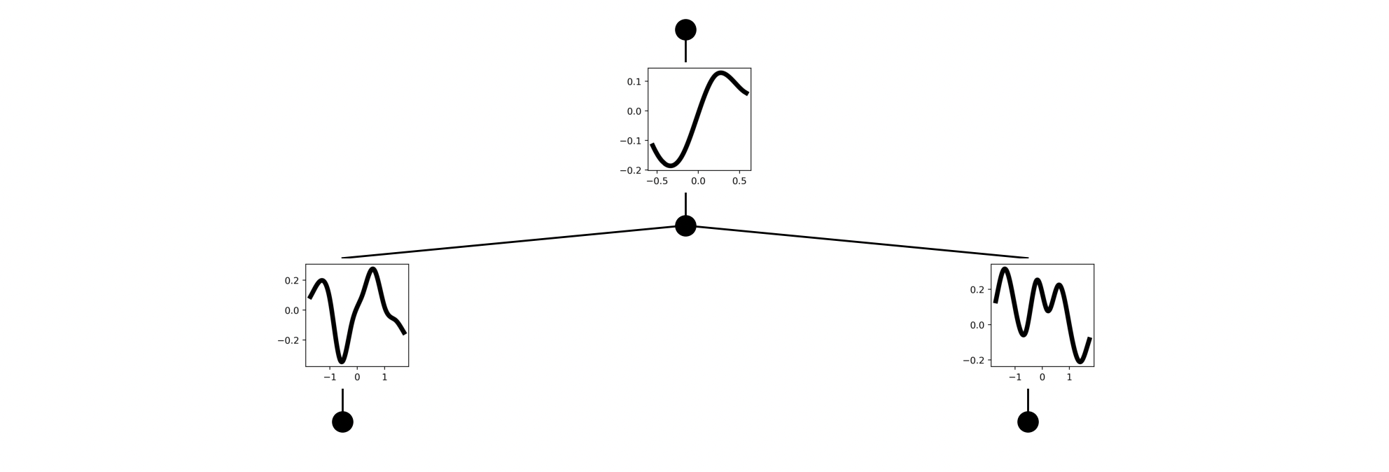
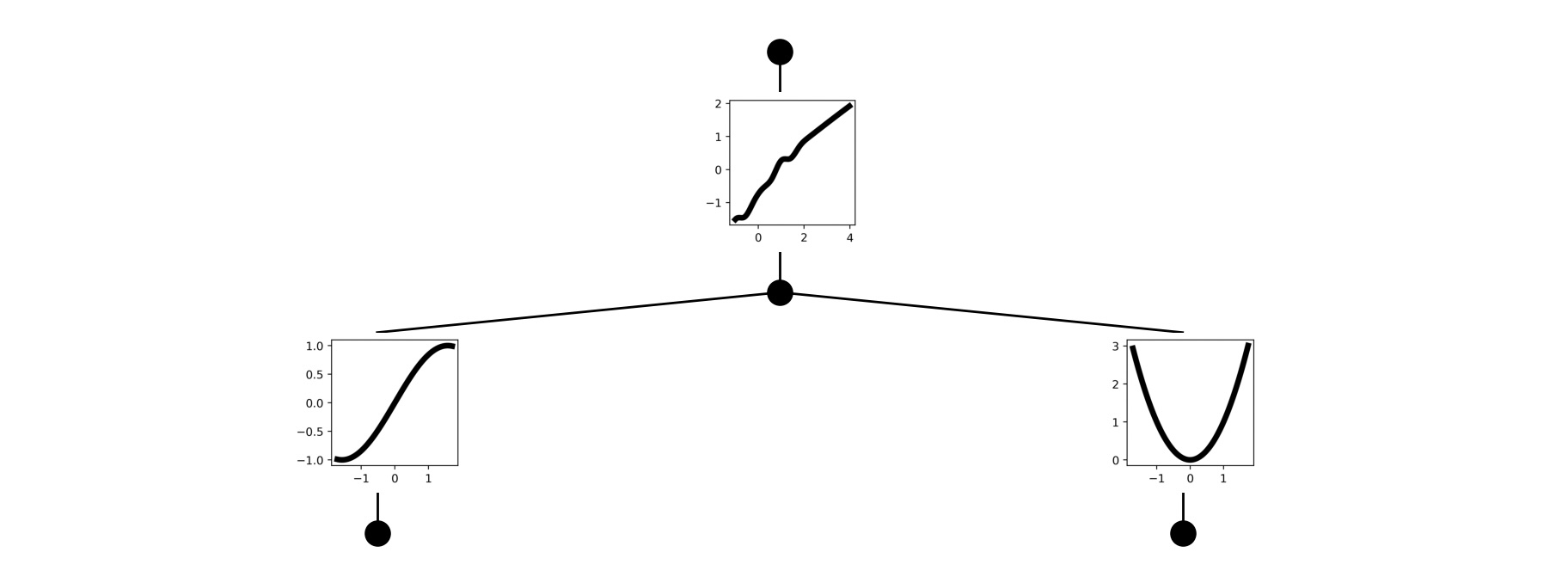
For example, we can visualize the base network activations with the script below.
f = lambda x: (torch.sin(x[:, [0]]) + x[:, [1]] ** 2)
dataset = create_dataset(f, n_var=2, train_num=1000, test_num=100)
# Initialize and plot KAN
config = KANConfig()
layer_widths = [2, 1, 1]
model = KAN(layer_widths, config)
model(dataset["train_input"])
plot(model)
Visualizing the activations of a randomly initialized KAN network.
Synthetic Example
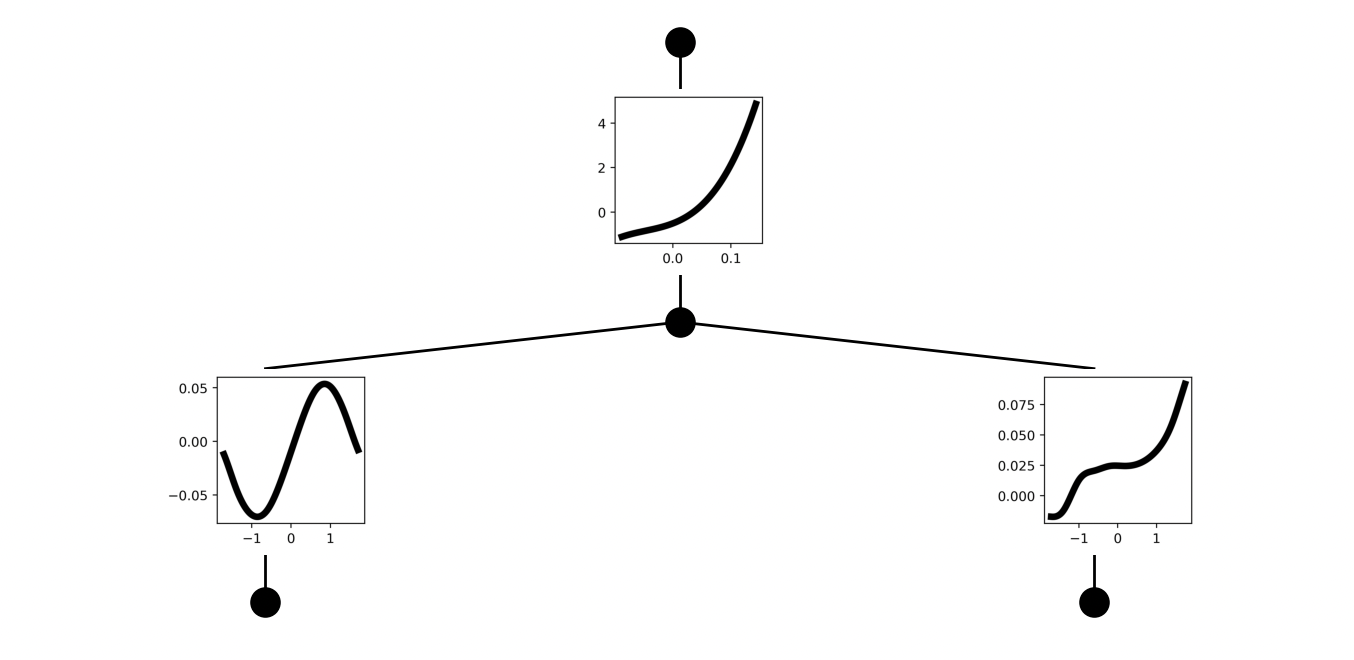
We can put this all together with a simple example. I would recommend scaling this further to a more interesting task, but for now you can verify that the model training is correct. Consider a function of the form \(f(x_1,x_2) = \exp \left( \sin(\pi x_1) + x_2^3 \right)\). We are going to learn this function using a KAN of the form \(f(x) = \mathcal{K}_{1,1} \left( \mathcal{K}_{1,2} \left( x_1, x_2 \right) \right)\).
Visualizing the activations of a trained KAN network. As expected, the activations learn (affine transformation of) the correct symbolic functions compose to form the original desired function.
Part III: KAN-specific Optimizations
The attentive reader may have noticed that the choice of B-spline is somewhat arbitrary, and the KAN itself is not necessarily tied to this choice of function approximator. In fact, B-splines are not the only choice to use, even among the family of different spline regressors. https://stats.stackexchange.com/questions/422702/what-is-the-advantage-of-b-splines-over-other-splines
A large portion of the original paper covers computation tricks to construct KANs with B-splines as the learnable activation function. While the authors prove a (type of) universal approximation theorem for KANs with B-splines, there are other choices of parameterized function classes that can be explored, potentially for computational efficiency.B-splines are defined over an interval, and evaluating B-spline functions on an input $x$ inherently requires branching logic because the basis functions are only non-zero over a certain interval. To take advantage of modern deep learning hardware, we would ideally like to use a representation that uses a minimal number of the same type of instruction (e.g. multiplication for MLPs) to compute the layer forward pass.
Remark. Because we are modifying the code from Part I, I’ve tried to keep the code compact by only including areas where changes were made. You can either follow along, or use the full KAN notebook.
B-Spline Optimizations: Grid Extension
Recall that the flexibility of our B-splines are determined by the number of learnable coefficients, and therefore the number of basis functions that it has. Furthermore, the number of basis functions is determined by the number of knot points \(G\). Suppose now that we want to include \(G'\) knots for a finer granularity on our learnable activations. Ideally, we want to add more knot points while preserving the original shape of the function. In other words, we want
We can tensorize this expression with respect to a batch of inputs $(z_1,…,z_b)$You may be confused why I use the variable $z$. Recall that we have a unique B-spline for every activation, or $m \times n$ of them. For edge $j \rightarrow i$, each $z_1,...,z_b$ would be each $x_j$ in the batch. Using $x_1,...,x_b$ would conflate the input vector $x$ and an individual coordinate of the input.
which is of the form $AX = B$. We can thus use least-square to solve for $X$, giving us our new coefficients on our finer set of knot points.
def grid_extension(self, x: torch.Tensor, new_grid_size: int):
"""
Increase granularity of B-spline activation by increasing the
number of grid points while maintaining the spline shape.
"""
# Re-generate grid points with extended size (uniform)
new_grid = generate_control_points(
self.grid_range[0],
self.grid_range[1],
self.in_dim,
self.out_dim,
self.spline_order,
new_grid_size,
self.device,
)
# bsz x out_dim x in_dim x (old_grid_size + spline_order)
old_bases = self.univarate_fn(x, self.grid, self.spline_order, self.device)
# bsz x out_dim x in_dim x (new_grid_size + spline_order)
bases = self.univarate_fn(x, new_grid, self.spline_order, self.device)
# out_dim x in_dim x bsz x (new_grid_size + spline_order)
bases = bases.permute(1, 2, 0, 3)
# bsz x out_dim x in_dim
postacts = torch.sum(old_bases * self.coef[None, ...], dim=-1)
# out_dim x in_dim x bsz
postacts = postacts.permute(1, 2, 0)
# solve for X in AX = B, A is bases and B is postacts
new_coefs = torch.linalg.lstsq(
bases.to(self.device),
postacts.to(self.device),
driver="gelsy" if self.device == "cpu" else "gelsd",
).solution
# Set new parameters
self.grid_size = new_grid_size
self.grid = new_grid
self.coef = torch.nn.Parameter(new_coefs, requires_grad=True)
I wanted to mention that for the driver parameter in torch.linalg.lstsq, there are certain solvers like QR decomposition that require full-rank columns on the basis functions. I’ve chosen to avoid these solvers, but there are several ways to go about solving the least-squares problem efficiently.
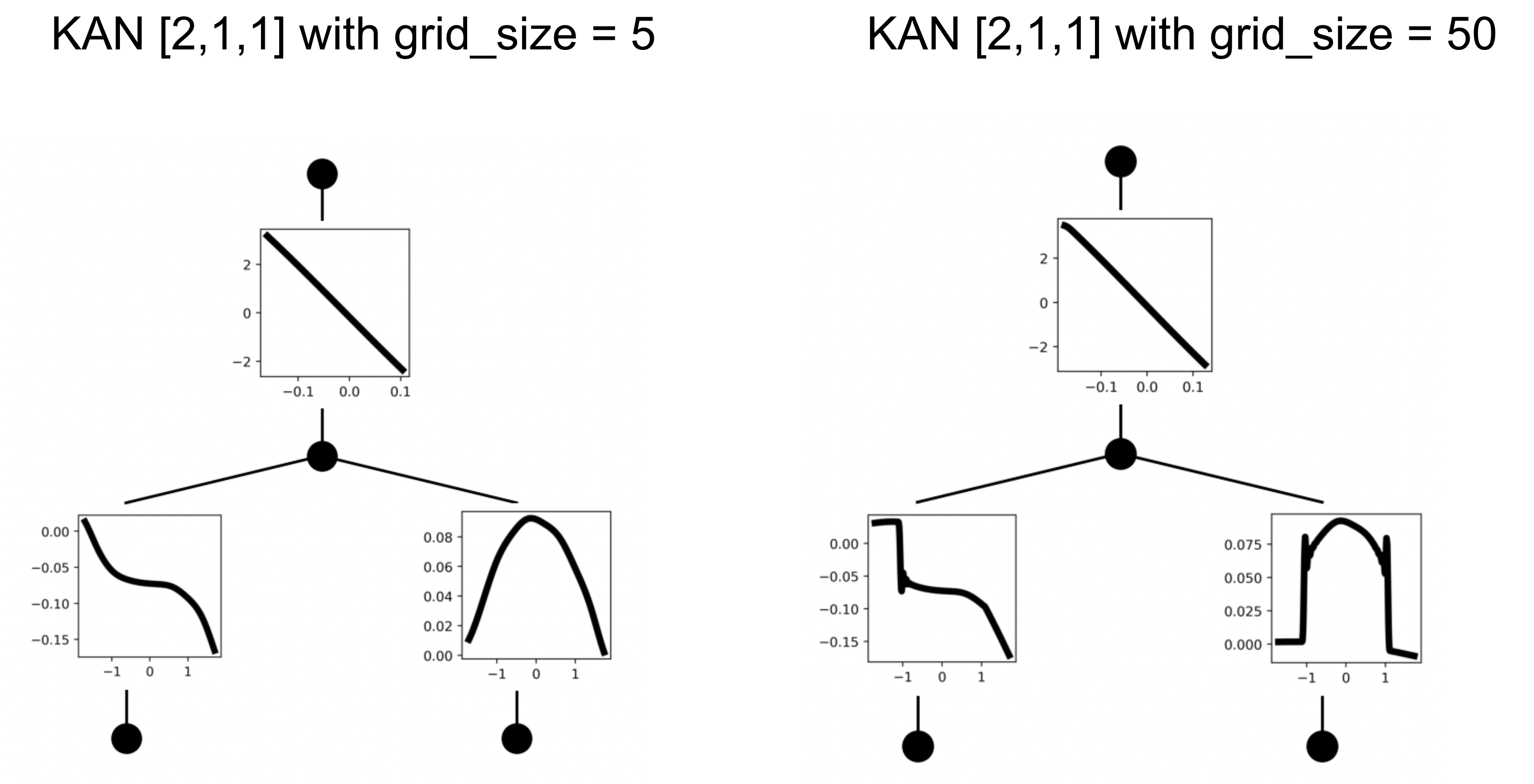
We can visually evaluate the accuracy of our grid extension algorithm by simply looking at the activations before and after a grid extension.
You will notice in the generated plot above that the KAN learns the correct function $$f(x_1,x_2) = (x_1^3 + x_2^2)$$. Grid extending from a grid size of 5 (left) to 50 (right) using least-squares. You can see some poor fitting behavior on the right activation, possibly due to an insufficient spread of data sampled for grid extension.
Activation Pruning
Pruning network weights is not unique to KANs, but they help the models become more readable and interpretable. Our implementation of pruning is going to be extremely inefficient, as we will mask out activations after they are calculated. There is already a large body of works for neural networks dedicated to bringing about performance benefits through pruningThere are both memory footprint and computation benefits to pruning. On the memory side, reducing the number of parameters is a clear benefit. On the compute side, specific pruning patterns like 2:4 pruning can be made into efficient kernels. Our implementation yields none of these benefits, and is only useful for interpreting the model. so we choose to make the code simple. To begin, we can first define a mask over the activations \(\mathcal{M}_{i,j} \in \{0,1\}^{m \times n}\) that zeros out activations belonging to pruned edges. In practice, we would want to prune before the computation, but tensorizing this process efficiently is not clean.
class KANLayer(nn.Module):
"Defines a KAN layer from in_dim variables to out_dim variables."
"Updated to include pruning mechanism."
def __init__(self, ...)
self.activation_mask = nn.Parameter(
torch.ones((out_dim, in_dim), device=device), requires_grad=False
) # <-- added mask
...
def forward(self, x: torch.Tensor):
...
# Form the batch of matrices phi(x) of shape [batch_size x out_dim x in_dim]
phi = self.residual_layer(x, spline)
# Mask out pruned edges
phi = phi * self.activation_mask[None, ...] # <-- added mask logic
...
We also need to define a metric for pruning. We can define this function at the high-level KAN module. For every layer, each node is assigned two scores: the input score is the absolute value of the maximum activation averaged over the training batch inputIdeally we want to pass in the entire training dataset when computing this, but it seems costly. For now, we just assume a large batch of data can sufficiently approximate the whole dataset., while the output score is computed the same, but for its output activations. More formally,
If \(\text{score}^{(\ell, \text{in})}_{i} < \theta \lor \text{score}^{(\ell, \text{out})}_{i} < \theta\) for some threshold $\theta = 0.01$, then we can prune the node by masking its incoming and outgoing activations. We tensorize this operation as a product of two indicators below.
class KAN(nn.Module):
...
@torch.no_grad
def prune(self, x: torch.Tensor, mag_threshold: float = 0.01):
"""
Prune (mask) a node in a KAN layer if the normalized activation
incoming or outgoing are lower than mag_threshold.
"""
# Collect activations and cache
self.forward(x)
# Can't prune at last layer
for l_idx in range(len(self.layers) - 1):
# Average over the batch and take the abs of all edges
in_mags = torch.abs(torch.mean(self.layers[l_idx].activations, dim=0))
# (in_dim, out_dim), average over out_dim
in_score = torch.max(in_mags, dim=-1)[0]
# Average over the batch and take the abs of all edges
out_mags = torch.abs(torch.mean(self.layers[l_idx + 1].activations, dim=0))
# (in_dim, out_dim), average over out_dim
out_score = torch.max(out_mags, dim=0)[0]
# Check for input, output (normalized) activations > mag_threshold
active_neurons = (in_score > mag_threshold) * (out_score > mag_threshold)
inactive_neurons_indices = (active_neurons == 0).nonzero()
# Mask all relevant activations
self.layers[l_idx + 1].activation_mask[:, inactive_neurons_indices] = 0
self.layers[l_idx].activation_mask[inactive_neurons_indices, :] = 0
In practice, you will call the prune(...) function after a certain number of training steps or post-training. Our current plotting function does not support these pruned activations, but we add this feature in the Appendix.
Fixing Symbolic Activations
A large selling point of the original paper is that KANs can be thought of as a sort of “pseudo-symbolic regression”. In some sense, if you know the original activations before-hand or realize that the activations are converging to a known non-linear function (e.g. $b \sin(x)$), we can choose to fix these activations. There are many ways to implement this feature, but similar to the pruning section, I’ve chosen to favor readability over efficiency. The original paper mentions two features that are not implemented below. Namely, storing coefficients affine transformations of known functions (e.g. $a f(b x + c) + d$) and fitting the current B-spline approximation to a known function. The code below allows the programmer to directly fix symbolic functions in the form of univariate Python lambda functions. First, we provide a function for a KAN model to fix (or unfix to the B-spline) a specific layer’s activation to a specified function.
class KAN(nn.Module):
...
@torch.no_grad
def set_symbolic(
self,
layer: int,
in_index: int,
out_index: int,
fix: bool,
fn,
):
"""
For layer {layer}, activation {in_index, out_index}, fix (or unfix if {fix=False})
the output to the function {fn}. This is grossly inefficient, but works.
"""
self.layers[layer].set_symbolic(in_index, out_index, fix, fn)
We first define a KANSymbolic module that is analogous to the KANActivation module used to compute B-spline activations. Here, we store an array of functions \(\{f_{i,j}(\cdot)\}_{i \in [m], j \in [n]}\) that are applied in the forward pass to form a matrix \(\{f_{i,j}(x_j)\}_{i \in [m], j \in [n]}\). Each function is initialized to be an identity function. Unfortunately, there is not (to my knowledge) an efficient way to perform this operation in the general case where all the symbolic functions are unique.
class KANSymbolic(nn.Module):
"Defines and stores the Symbolic functions fixed / set for a KAN."
def __init__(self, in_dim: int, out_dim: int, device: torch.device):
"""
We have to store a 2D array of univariate functions, one for each
edge in the KAN layer.
"""
super(KANSymbolic, self).__init__()
self.in_dim = in_dim
self.out_dim = out_dim
self.fns = [[lambda x: x for _ in range(in_dim)] for _ in range(out_dim)]
def forward(self, x: torch.Tensor):
"""
Run symbolic activations over all inputs in x, where
x is of shape (batch_size, in_dim). Returns a tensor of shape
(batch_size, out_dim, in_dim).
"""
acts = []
# Really inefficient, try tensorizing later.
for j in range(self.in_dim):
act_ins = []
for i in range(self.out_dim):
o = torch.vmap(self.fns[i][j])(x[:,[j]]).squeeze(dim=-1)
act_ins.append(o)
acts.append(torch.stack(act_ins, dim=-1))
acts = torch.stack(acts, dim=-1)
return acts
def set_symbolic(self, in_index: int, out_index: int, fn):
"""
Set symbolic function at specified edge to new function.
"""
self.fns[out_index][in_index] = fn
We now have to define the symbolic activation logic inside the KAN layer. When computing the output activations, we use a similar trick to the pruning implementation by introducing a mask that is $1$ when the activation should be symbolicRemember that this solution has the same inefficiencies as the pruning solution. We end up computing activations for both the B-splines and the symbolic activations. For readability, we've chosen to implement it this way, but in practice you will probably want to change this. and $0$ when it should be the B-spline activation. We also add the function for setting an activation to be a symbolic function and modify the forward pass to support this operation.
We learn a [2,1,1] KAN for the function $$f(x_1,x_2) = \sin(x_1) + x_2^2$$, but we fix the first layer to have symbolic activations using a lambda function.
Part IV: Applied Example
This section will be focused on applying KANs to a standard machine learning problem. The original paper details a series of examples where KANs learn to fit a highly non-linear or compositional function. Of course, while these functions are difficult to learn, the use of learnable univariate functions makes KANs suitable for these specific tasks. I emphasized the similarities between KANs and standard deep learning models throughout this post, so I also wanted to present a deep learning example (even though it doesn’t work very well). We will run through a simple example of training a KAN on the canonical MNIST handwritten digits dataset to show how easy it is to adapt these models for standard deep learning settings. We first download the relevant data.
# Run these without ! in terminal, or run this cell if using colab.
!wget www.di.ens.fr/~lelarge/MNIST.tar.gz
!tar -zxvf MNIST.tar.gz -C data/
In the interest of reusing the existing train logic we created earlier, we write a function to turn a torch.Dataset with MNIST into the dictionary format. For general applications, I recommend sticking with the torch Dataloader framework.
def split_torch_dataset(train_data, test_data):
"""
Quick function for splitting dataset into format used
in rest of notebook. Don't do this for your own code.
"""
dataset = {}
dataset['train_input'] = []
dataset['train_label'] = []
dataset['test_input'] = []
dataset['test_label'] = []
for (x,y) in train_data:
dataset['train_input'].append(x.flatten())
dataset['train_label'].append(y)
dataset['train_input'] = torch.stack(dataset['train_input']).squeeze()
dataset['train_label'] = torch.tensor(dataset['train_label'])
dataset['train_label'] = F.one_hot(dataset['train_label'], num_classes=10).float()
for (x,y) in test_data:
dataset['test_input'].append(x.flatten())
dataset['test_label'].append(y)
dataset['test_input'] = torch.stack(dataset['test_input']).squeeze()
dataset['test_label'] = torch.tensor(dataset['test_label'])
dataset['test_label'] = F.one_hot(dataset['test_label'], num_classes=10).float()
print('train input size', dataset['train_input'].shape)
print('train label size', dataset['train_label'].shape)
print('test input size', dataset['test_input'].shape)
print('test label size', dataset['test_label'].shape)
return dataset
Finally, like all previous examples, we can run a training loop over the MNIST dataset. We compute the training loss using the standard binary cross-entropy loss and define the KAN to produce logits from 0-9. Due to restrictions in our train() function, we define our test loss as the total number of incorrectly marked samples out of $100$ validation samples.
You may notice that the training is significantly slower even for such a small model. Furthermore, the results here are not good as expected. I’m confident that with sufficient tuning of the model you can get MNIST to work (there are examples of more sophisticated KAN implementations that perform extremely well), but the above example raises questions about the efficiency of the original implementation. Before we are able to properly scale these models, we need to first study the choice of parameterization and whether we should even treat KANs the way we treat MLPs.
Conclusion
I hope this resource was useful to you – whether you learned something new, or gained a certain perspective along the way. I wrote up this annotated blog to clean up my notes on the topic, as I am interested in improving these models from an efficiency perspective. If you find any typos or have feedback about this resource, feel free to reach out!
Appendix
I may re-visit this section in the future with some more meaningful experiments when I get the time.
Plotting Symbolic and Pruned KANs
The plotting function defined in Network Visualization doesn’t include logic for handling the pruned activation masks and the symbolic activations. We will include this logic separately, or you can follow the rest of the visualization code in the original repository.
Open Research: Making KANs Efficient
It is known that these models currently do not scale well due to both memory and compute inefficiencies. Of course, it is unknown whether scaling these models will be useful, but the authors posit that they are more parameter efficient than standard deep learning models because of the flexibility of their learned univariate functions. As you saw in the MNIST example, it is not easy to scale the model even for MNIST training. I sort of avoided this question before, but I want to highlight a few reasons for these slowdowns.
We fully materialize a lot of intermediate activations for the sake of demonstration, but even in an optimized implementation, some of these intermediate activations are unavoidable. Generally, materializing intermediate activations means lots of movement between DRAM and the processors, which can cause significant slowdown. There is a repository called KAN-benchmarking dedicated to evaluating different KAN implementations. I may include an extra section on profiling in the future.
Each activation \(\Phi_{i,j}\) or edge in the network is potentially different. At an machine instruction level, this means that we cannot take advantage of SIMD or SIMT that standard GEMM or GEMV operations have on the GPU. There are alternative implementations of KANs that were mentioned earlier that attempt to get around these issues , but even then they do not scale well compared to MLPs. I suspect the choice of the family of parameterized activations will be extremely important moving forward.
B-Spline Optimizations: Changing Knot Points
A natural question is whether we have to fix the knot points to be uniformly spaced, or if we can use the data to adjust our knot points. The original paper does not detail this optimization, but their codebase actually includes this feature. If time permits, I may later include a section on this – I think it may be important for performance of KANs with B-splines, but for general KANs maybe not.
Citation
Just as a formality, if you want to cite this for whatever reason, use the BibTeX below.
@article{zhang2024annotatedkan,
  title   = "Annotated KAN",
  author  = "Zhang, Alex",
  year    = "2024",
  month   = "June",
  url     = "https://alexzhang13.github.io/blog/2024/annotated-kan/"
}